Creating a Day Index in Excel and Google Sheets
A fun challenge that I faced a few days was creating a weekday/weekend day index in Google sheets to count and index the number of weekdays/weekends in a month. This might sound like something easily achieved by placing a static value next to the date based on the preceding index value and day of the week, but the more this process has to be replicated, the more boring and tedious the task will become. This process is simply not for me as I hate manual excel work. As a result, I decided to take
Excerpt
A fun challenge that I faced a few days was creating a weekday/weekend day index in Google sheets to count and index the number of weekdays/weekends in a month. This might sound like something easily achieved by placing a static value next to the date based on the preceding index value and day of the week, but the more this process has to be replicated, the more boring and tedious the task will become. This process is simply not for me as I hate manual excel work. As a result, I decided to take some additional time to create an automated way to index and reset the index at the start of the month using a single formula. In the rest of this post, I will provide you with a step by step outline on how you can replicate my formula within your own work and save you from this spreadsheet grunt work. I hope you will find this guide useful and think of interesting ways of repurposing the formula for non-date related functions!
Goal: Create an auto incrementing system to individually index the position of the weekday or weekend within the month. This indexing should reset at the start of a new month without modification to the formula.
Excel / Google Sheets functions Involved:
-
WEEKDAY() -
OR() -
IF() -
SUMIFS() -
EOMONTH()
Step 1
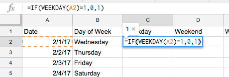
Add in the dates that should be indexed, as well as two columns for converting the date into weekday/weekend cohorts. In order to get these cohorts, we must convert the date column into a sequential number that represents the day of the week for that day within the specific year used. This is done with the `WEEKDAY()` function, which converts a date into a number starting from 1 (or 0) to 7 (or 6). What each number represents when using this function is based on the “Return_type” you provide it. By default it starts with 1 representing Sunday and goes until 7, which represents Saturday. We will use this order for our formula.
=WEEKDAY(A2)
Step 2
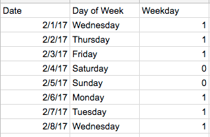
Now that we have a sequential order in place, we need to layer in a way to identify the dates that exist on a weekend versus those that exist on a weekday. To do this, we use an `IF()` function to look at the weekday value and then provide a 1 if it is a weekday and 0 if it is a weekend. This process should be replicated in a second column to get the inverse of the previous columns statement. i.e. a 1 if it is a weekend and a 0 if it is a weekday.
=IF(WEEKDAY(A2)=1,0,1) //Outputs one if date is a number between 2-7 (Monday-Saturday) and zero if it is a Sunday
However, you will immediately notice that the evaluation portion of the function only handles one value and we need it to fit two values, 1, representing Sunday and 7 representing Saturday. In order to build on what we have, we replace the evaluation portion with an OR() statement that says if WEEKDAY()=1 OR WEEKDAY()=7, then place a value of 1 or 0 depending on which is in the “true” portion of the function.
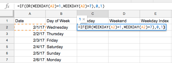
=IF(OR(WEEKDAY(A2)=1,WEEKDAY(A2)=7),0,1) //outputs one if date is a weekday and zero if date is a weekend
Step 3
With two columns in place containing dummy variables representing the weekday and weekend cohorts for each of our dates, it is now time to create our day index columns for the weekday and weekend. When conceptualizing the formula, make sure to think about all of the criteria that should be evaluated before outputting a value. In the case of this day index, we need to know if the date is a weekday or a weekend, the month that the date lands in, how far into the month that date is and the day on which the month ends.
This definitely sounds like a lot, but we can break it down into different parts before putting it all together.
The first thing we want to do is figure out how to aggregate the weekday/weekend dummy variable column if certain criteria is matched. To do this, we will use the SUMIFS() function. The sum portion of this function should be self-evident, but if it isn’t :) , it should be one of the dummy variable columns we used to create weekday / weekend cohorts.
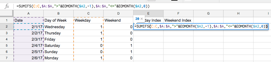
Next, we will add three criteria to aggregate only those values that exist on a date, which is greater than the first day of the month, less than or equal to the last day of the month, and only those days that exist before or occur on the criteria date. For all of these conditions, we will use the date column as the criteria range.
Greater than the first day of the month
=SUMIFS(Output, Array, ">"&EOMONTH(LookupValue,-1))
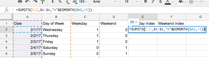
Please that 23 represents the number of ones in this column greater than 1/31/17 and up to 3/5/17, which is where I stopped my date.
Less than or equal to the last day of the month
=SUMIFS(Output, Array, ">"&LookupValue, Array, "<="&EOMONTH(LookupValue,-1))
This value has dropped by decremented by three because 3/1/17 - 3/3/17 (All weekday’s) have been excluded because it is greater than the month of the current date.
Exist before or occur on the criteria date
=SUMIFS(Output, Array, ">"&EOMONTH(LookupValue,-1)), Array, "<="&LookupValue, Array, "<="&EOMONTH(LookupValue,0))
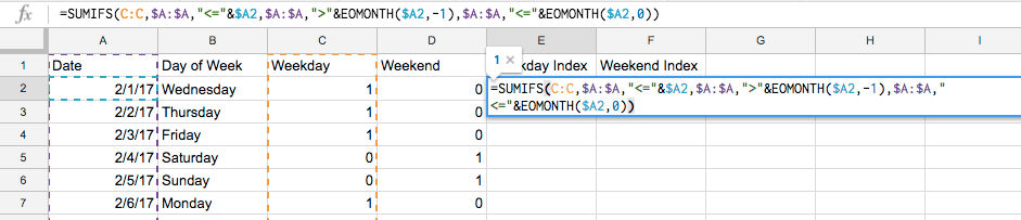
*With this final criteria, we are saying that we should only sum those values that are equal to or less than the current date. *
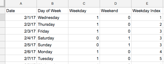
And with that, we complete our indexing criteria. You now have an auto incrementing day index that resets at the start of each month...However, there is one more step that needs to take place.
Step 4
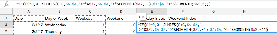
With our current formula, if a row within our dummy variable columns contains a zero, then it will simply copy the last summed value in its place until a new one value is found. In order to clean this up and visually display breaks in our index, we will enclose our formula in an `IF()` function. This will look at the either the weekday or weekend column and if the value is equal to zero, set the value as zero, otherwise continue with our day index formula. Once this is in place, we have officially completed the day indexing formula.
=IF(Weekday/Weekend LookupValue = 0, 0, SUMIFS(Output, Array, ">"&EOMONTH(LookupValue,-1)), Array, "<="&LookupValue, Array, "<="&EOMONTH(LookupValue,0)))
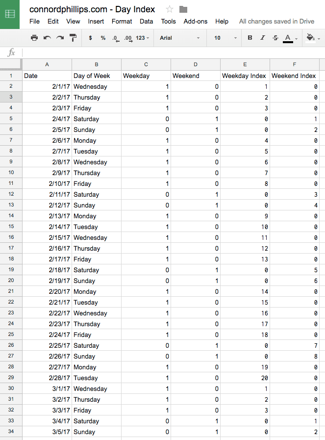
Result:
Now Automate, Automate, Automate
I hope you have found this guide helpful in turning a tedious task into a pluggable formula that can streamline day indexing requests. While this formula was originally built for this specific workflow, the structure of the formula is flexible enough to be repurposed for non-date specific indexing. All that is really needed to do so are a set of dummy variables for each filtering criteria that is provided.
Now go ahead and apply it to your reports and then think about all of the time you have saved by having this formula in your tool belt!